\(\)
Problem 6-12
Assume that \(V(\mathbf{r})\) is independent of time and show that the time integral of the second-order scattering term \(K^{(2)}(b, a)\) gives
\def\mb#1{\mathbf{#1}}
K^{(2)}(b,a)&=\left(\frac{m}{2\pi\hbar^{2}}\right)^{2}\left(\frac{m}{2\pi i\hbar T}\right)^{3/2}\int d^{3}\mb{r}_c\int d^{3}\mb{r}_d\,
\frac{r_{c d}+r_{a c}+r_{b d}}{r_{c d}r_{a c}r_{b d}}\\
&\quad \times \left[ \exp\left(\frac{i m}{2\hbar T}\right)(r_{c d}+r_{a c}+r_{b d})^{2}\right]\,V(\mb{r}_{c})V(\mb{r}_{d})
\tag{6-58}
\end{align}
where the points \(a,b,c\) and \(d\) are arranged as shown in Fig. 6-9. The term \(r_{c d}\) stands for the distance between the point \(c\) and \(d\), etc. Assume that \(V(\mb{r})\) becomes negligibly small at distances which are short compared to \(R_{a}\) or \(R_{b}\). Show that the cross section is given by \(d\sigma/d\Omega = |f(\mb{q})|^{2}\) , where the scattering amplitude \(f(\mb{q})\), including the first-order term, is
f(\mb{q})&=-\frac{m}{2\pi \hbar^{2}}\int d^{3}\mb{r}\,e^{-i\mb{p}_{a}\cdot\mb{r}/\hbar} \\
& + \left(\frac{m}{2\pi\hbar^{2}}\right)^{2}\int d^{3}\mb{r}_{c}\int d^{3}\mb{r}_{d}\,
e^{-i\mb{p}_{b}\cdot\mb{r}_{d}} V(\mb{r}_{d})\left(\frac{1}{r_{cd}}\right)\,e^{ipr_{cd}/\hbar}\,V(\mb{r}_{c})\,e^{i\mb{p}_{b}\cdot\mb{r}_{c}}
+ ( \mathrm{higher}\ \mathrm{order}\ \mathrm{terms} )
\tag{6-56}
\end{align}
where \(\mb{p}_{b}\) is the momentum of the electron traveling in the direction of \(\mb{R}_{b}\) and \(\mb{p}_{a}\) is the momentum of an electron traveling in the direction \(-\mb{R}_{a}\). The magnitude of the momentum is \(p\), and it is approximately unchanged by an elastic scattering of the electron from the ( relatively massive ) atom.
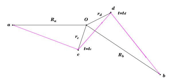
(Fig. 6-9) To increase the accuracy of scattering calculations, we can take account of second-order terms in the perturbation expansion.
Here, as in Fig. 6-2 (3), we picture the electron as being scattered at two separate points in the atomic potential. Thus the electron starts at \(a\); proceeds as a free particle to \(c\), where it is scattered; then moves as a free particle to \(d\), where it is scattered again; and finally moves as a free particle to \(b\), where it is collected by the counter. The points \(c\) and \(d\) can lie at any position in space. The atomic potential at these positions depends upon the radius vectors \(\mathbf{r}_c\) and \(\mathbf{r}_d\), measured from the center of the atom \(O\).
(解答例) 式 (6-17) から,2 次の散乱項 \(K^{(2)}(b,a)\) は次である:
K^{(2)}(b,a)=\left(-\frac{i}{\hbar}\right)^{2}\int d\tau_d\int d\tau_c\,K_0(b,d)\,V(d)\,K_0(d,c)\,
V(c)\,K_0(c,a)
\tag{1}
\end{equation}
ここで \(d\tau=dtd\mathbf{r}\) とする.( 原書では, § 6-1 の一般的な摂動展開を議論での図 6-2 と,この問題の配置図 6-9 で点 \(c\) と点 \(d\) の位置が逆になっているので注意する! ).
式 (6-33) の \(K^{(1)}\) を求めたときと同様に考えて, 自由粒子核 \(K_0(b,c),\,K_0(c,d),\,K_0(d,a)\) の各々は式 (3-52) を 3 次元化したものを用いて次とする:
K_0(b,d)&=\left(\frac{m}{2\pi i\hbar(T-t_d)}\right)^{3/2}\exp\left[\frac{im(\mb{R}_b-\mb{r}_d)^{2}}
{2\hbar(T-t_d)}\right],\\
K_0(d,c)&=\left(\frac{m}{2\pi i\hbar(t_d-t_c)}\right)^{3/2}\exp\left[\frac{im(\mb{r}_d
-\mb{r}_c)^{2}}{2\hbar(t_d-t_c)}\right],\\
K_0(c,a)&=\left(\frac{m}{2\pi i\hbar t_c}\right)^{3/2}\exp\left[\frac{im(\mb{r}_c-\mb{R}_a)^{2}}{2\hbar t_c}\right]
\tag{2}
\end{align}
ただし時間については, 暗黙の内に \(t_d>t_c\) を仮定しているので \(t_c\) の時間積分範囲は \(t_c=[0,t_d]\) とし,\(t_d\) の時間積分範囲は \(t_d=[0,T]\) とすればよい.また,\(r_{b d}\equiv \mb{R}_b-\mb{r}_d\),\(r_{d c}\equiv \mb{r}_d-\mb{r}_c\),\(r_{c a}\equiv \mb{r}_c-\mb{R}_a\) と表記し直すことにする.これらを式 (1) に適用すると次となる:
&K^{(2)}(b,a)=\left(-\frac{i}{\hbar}\right)^{2}\int d^{3}\mb{r}_d\int d^{3}\mb{r}_c\,
\int_0^{T}dt_d\int_0^{t_d}dt_c\,\left(\frac{m}{2\pi i\hbar(T-t_d)}\right)^{3/2}
\exp\left[\frac{i m r_{bd}^{2}}{2\hbar(T-t_d)}\right]V(\mb{r}_d)\\
&\quad\times\left(\frac{m}{2\pi i\hbar(t_d-t_c)}\right)^{3/2}\exp\left[\frac{i m r_{dc}^{2}}{2\hbar(t_d-t_c)}\right]V(\mb{r}_c)
\left(\frac{m}{2\pi i\hbar t_c}\right)^{3/2}\exp\left[\frac{i m r_{ca}^{2}}{2\hbar t_c}\right]
\tag{3}
\end{align}
まず \(dt_c\) についての時間積分 \(I_1\) を実施する:
I_1&=\int_0^{t_d}dt_c\,\left(\frac{m}{2\pi i\hbar(t_d-t_c)}\right)^{3/2}
\left(\frac{m}{2\pi i\hbar t_c}\right)^{3/2}\exp\left[\frac{i m r_{dc}^{2}}{2\hbar(t_d-t_c)}\right]
\exp\left[\frac{i m r_{ca}^{2}}{2\hbar t_c}\right]\\
&=\left(\frac{m}{2\pi i\hbar}\right)^{3}\int_0^{t_d}\exp\left[
-\frac{mr_{dc}^{2}}{2\hbar i\,(t_d-t_c)}-\frac{mr_{ca}^{2}}{2\hbar i\,t_c}\right]
\frac{dt_c}{\left[\sqrt{(t_d-t_c)t_c}\right]^{3}}
\end{align}
巻末付録の「役立つ定積分」の公式 (A-5) を用いる.この場合の \(a,\,b\) は,
a=\frac{mr_{dc}^{\ 2}}{2\hbar i},\quad b=\frac{mr_{ca}^{\ 2}}{2\hbar i}\quad \rightarrow\
\sqrt{a}+\sqrt{b}=\sqrt{\frac{m}{2\hbar i}}(r_{dc}+r_{ca}),\ \sqrt{ab}=\frac{m}{2\hbar i}r_{dc}r_{ca}
\end{equation}
従って,
I_1=\left(\frac{m}{2\pi i\hbar}\right)^{3}\frac{2\hbar i}{m}\sqrt{\frac{m}{2\hbar i}}
\sqrt{\frac{\pi}{t_d^{3}}}\frac{r_{dc}+r_{ca}}{r_{dc}r_{ca}}\exp\left[\frac{im}{2\hbar t_d}(r_{dc}+r_{ca})^{2}\right]
\tag{4}
\end{equation}
この結果を式 (3) に代入し, 今度は \(dt_d\) についての時間積分を行う.やはり公式 (A-5) を同様に用いると次となる:
I_2&=\frac{i^{2}}{\hbar^{2}}\int_0^{T}dt_d\,\left(\frac{m}{2\pi i\hbar(T-t_d)}\right)^{3/2}
\exp\left[\frac{i m r_{bd}^{2}}{2\hbar(T-t_d)}\right]\\
&\qquad\qquad\qquad\times\left(\frac{m}{2\pi i\hbar}\right)^{3}
\frac{2\hbar i}{m}\sqrt{\frac{m}{2\hbar i}}\sqrt{\frac{\pi}{t_d^{3}}}
\frac{r_{dc}+r_{ca}}{r_{dc}r_{ca}}\exp\left[\frac{im}{2\hbar t_d}(r_{dc}+r_{ca})^{2}\right]\\
&=\frac{i^{2}}{\hbar^{2}}\left(\frac{m}{2\pi i\hbar}\right)^{3/2}\frac{2\hbar i}{m}
\left(\frac{m}{2\pi i\hbar}\right)^{3}\sqrt{\frac{m\pi}{2\hbar i}}\frac{r_{dc}+r_{ca}}{r_{dc}r_{ca}}\\
&\qquad\qquad\qquad\times \int_0^{T}\exp\left[-\frac{mr_{bd}^{2}}{2\hbar i\,(T-t_d)}
-\frac{m(r_{dc}+r_{ca})^{2}}{2\hbar i\,t_d}\right]\frac{dt_d}{\left[\sqrt{(T-t_d)t_d}\right]^{3}}\\
&=\frac{i^{2}}{\hbar^{2}}\left(\frac{m}{2\pi i\hbar}\right)^{3/2}\frac{2\hbar i}{m}
\left(\frac{m}{2\pi i\hbar}\right)^{3}\sqrt{\frac{m\pi}{2\hbar i}}\frac{r_{dc}+r_{ca}}{r_{dc}r_{ca}}\\
&\qquad\qquad\qquad\times \frac{2\hbar i}{m}\sqrt{\frac{m\pi}{2\hbar i\,T^{3}}}
\frac{r_{bd}+r_{dc}+r_{ca}}{r_{bd}(r_{dc}+r_{ca})}\exp\left[\frac{im}{2\hbar T}(r_{bd}+r_{dc}+r_{ca})^{2}\right]\\
&=\left(-\frac{m}{2\pi\hbar^{2}}\right)^{2}\left(\frac{m}{2\pi i\hbar T}\right)^{3/2}
\frac{r_{bd}+r_{dc}+r_{ca}}{r_{bd}r_{dc}r_{ca}}\exp\left[\left(\frac{im}{2\hbar T}\right)
(r_{bd}+r_{dc}+r_{ca})^{2}\right]
\tag{5}
\end{align}
これを式 (3) に代入すると,\(K^{(2)}\) が式 (6-58) のように得られる:
K^{(2)}(b,a)&=\left(-\frac{m}{2\pi\hbar^{2}}\right)^{2}\left(\frac{m}{2\pi i\hbar T}\right)^{3/2}
\int d^{3}\mb{r}_c\int d^{3}\mb{r}_d\,\frac{r_{bd}+r_{dc}+r_{ca}}{r_{bd}r_{dc}r_{ca}}\\
&\qquad\qquad\times\exp\left[\left(\frac{im}{2\hbar T}\right)(r_{bd}+r_{dc}+r_{ca})^{2}\right]
V(\mb{r}_c)\,V(\mb{r}_d)
\tag{6-58}
\end{align}
今度は,2次までの散乱振幅 \(f(\mb{q})=f^{(1)}(\mb{q})+f^{(2)}(\mb{q})\) を考える.ただし \(f^{(1)}(\mb{q})\) は式 (6-44) 中のものである:
\frac{d\sigma(\theta)}{d\Omega}=\left| f^{(1)}(\mb{q})\right|^{2}
=\left|-\frac{m}{2\pi\hbar^{2}}v(\mb{q})\right|^{2}
\tag{6.44′}
\end{equation}
\(f^{(2)}(\mb{q})\) は式 (6-42) を求めたときと同様な議論により求められる.ただし式 (6-58) の \(K^{(2)}(b,a)\) に等価な式に於いては \(r_{d c}\ll r_{b d},\,r_{c a}\) なので, 次のような近似を用いよう:
\def\reverse#1{\frac{1}{#1}}
\frac{r_{bd}+r_{dc}+r_{ca}}{r_{bd}r_{dc}r_{ca}}&\simeq \reverse{r_{dc}}\frac{r_{bd}+r_{ca}}{r_{bd}r_{ca}}
=\reverse{r_{dc}}\left(\reverse{r_{ca}}+\reverse{r_{bd}}\right)\\
&\simeq \reverse{r_{dc}}\left(\reverse{r_a}+\reverse{r_{b}}\right)
\tag{6}
\end{align}
すると \(K^{(2)}\) は, 近似的に次のように書くことが出来る:
&K^{(2)}(b,a)\simeq\left(-\frac{m}{2\pi\hbar^{2}}\right)^{2}
\left(\frac{m}{2\pi i\hbar T}\right)^{3/2}\left(\reverse{r_a}+\reverse{r_{b}}\right)\times I_2\\
&\quad\text{where}\quad I_2=\int d^{3}\mb{r}_c\int d^{3}\mb{r}_d\,\reverse{r_{dc}}\exp\left[\left(
\frac{im}{2\hbar T}\right)(r_{bd}+r_{dc}+r_{ca})^{2}\right]V(\mb{r}_c)\,V(\mb{r}_d)
\tag{7}
\end{align}
この絶対値の 2 乗 \(|K^{(2)}(b,a)|^{2}\) と \(|K_0(b,a)|^{2}\) は,
\Bigl|K^{(2)}(b,a)\Bigr|^{2}&=\left(-\frac{m}{2\pi\hbar^{2}}\right)^{4}\left|
\frac{m}{2\pi i\hbar T}\right|^{3}\frac{(r_a+r_b)^{2}}{r_a^{2}r_b^{2}}\times I_2^{2},\\
\Bigl|K_0(b,a)\Bigr|^{2}&=\left|\left(\frac{m}{2\pi i \hbar T}\right)^{3/2}\right|^{2}=\left|\frac{m}{2\pi i\hbar T}\right|^{3}
\end{align}
となるから, 式 (6-42) を求めたときと同様にして次が得られる:
\frac{P(b)}{P(d)}&=\left|\frac{K^{(2)}(b,a)}{K_0(b,a)}\right|^{2}
=\left(-\frac{m}{2\pi\hbar^{2}}\right)^{4}I_2^{2}\times \frac{(r_a+r_b)^{2}}{r_a^{2}r_b^{2}}\\
&=\left(\frac{m}{2\pi\hbar^{2}}\right)^{2}\left|-\frac{m}{2\pi\hbar^{2}}I_2\right|^{2}\frac{(r_a+r_b)^{2}}{r_a^{2}r_b^{2}}
\end{align}
従って, 式 (6-42) との比較から, この場合の \(|v(\mb{q})|^{2}\) に相当するのは次である:
\left|v^{(2)}(\mb{q})\right|^{2}=\left|-\frac{m}{2\pi\hbar^{2}}I_2\right|^{2}\quad
\rightarrow\quad v^{(2)}(\mb{q})=-\frac{m}{2\pi\hbar^{2}}I_2
\tag{8}
\end{equation}
従って, 式 (6-44′) との類推で,2次のボルン散乱振幅 \(f^{(2)}(\mb{q})\) は次とすることが出来る:
&f^{(2)}(\mb{q})=-\frac{m}{2\pi\hbar^{2}}v^{(2)}(\mb{q})
=\left(-\frac{m}{2\pi\hbar^{2}}\right)\times \left(-\frac{m}{2\pi\hbar^{2}}\right)I_2\\
&=\left(-\frac{m}{2\pi\hbar^{2}}\right)^{2}\int d^{3}\mb{r}_c\int d^{3}\mb{r}_d\,\reverse{r_{dc}}
\exp\left[\left(\frac{im}{2\hbar T}\right)(r_{bd}+r_{dc}+r_{ca})^{2}\right]V(\mb{r}_c)\,V(\mb{r}_d)
\tag{9}
\end{align}
更に指数関数中の量 \((r_{b d}+r_{d c}+r_{c a})^{2}\) は, \(r_{d c}\ll r_{b d},\,r_{c a}\) であることに注意する.また,
r_{b d}\simeq R_b-\mb{i}_b\cdot\mb{r}_d,\qquad\text{and}\qquad r_{c a}\simeq R_a+\mb{i}_a\cdot\mb{r}_c
\end{equation}
とすることで, 次のように近似できる:
&(r_{b d}+r_{d c}+r_{c a})^{2}\simeq (r_{b d}+r_{c a})^{2}+2r_{d c}(r_{b d}+r_{c a})
=(r_{b d}+r_{c a})(r_{b d}+r_{c a}+2r_{d c})\\
&=(R_b+R_a+\mb{i}_a\cdot\mb{r}_c-\mb{i}_b\cdot\mb{r}_d)(R_b+R_a+\mb{i}_a\cdot\mb{r}_c-\mb{i}_b\cdot
\mb{r}_d+2r_{dc})\\
&=(R_a+R_b)^{2}+2(R_a+R_b)(\mb{i}_a\cdot\mb{r}_c-\mb{i}_b\cdot\mb{r}_d)\\
&\quad+(\mb{i}_a\cdot\mb{r}_c-\mb{i}_b\cdot\mb{r}_d)^{2}+2(R_a+R_b)r_{dc}
+2r_{dc}(\mb{i}_a\cdot\mb{r}_c-\mb{i}_b\cdot\mb{r}_d)\\
&\simeq (R_a+R_b)^{2}+2(R_a+R_b)(\mb{i}_a\cdot\mb{r}_c-\mb{i}_b\cdot\mb{r}_d+r_{dc})
\tag{10}
\end{align}
すると式 (9) の積分部分 \(I_2\) は, 次のように近似して書くことが出来る:
I_2&=\int d^{3}\mb{r}_c\int d^{3}\mb{r}_d\,\reverse{r_{dc}}
\exp\left[\left(\frac{im}{2\hbar T}\right)(r_{bd}+r_{dc}+r_{ca})^{2}\right]V(\mb{r}_c)\,V(\mb{r}_d)\\
&=\int d^{3}\mb{r}_c\int d^{3}\mb{r}_d\,\frac{V(\mb{r}_c)\,V(\mb{r}_d)}{r_{dc}}
\exp\left[\left(\frac{im}{2\hbar T}\right)\left\{(R_a+R_b)^{2}+2(R_a+R_b)(\mb{i}_a\cdot\mb{r}_c
-\mb{i}_b\cdot\mb{r}_d+r_{dc})\right\}\right]\\
&=\exp\left[\left(\frac{im}{2\hbar T}\right)(R_a+R_b)^{2}\right]\int d^{3}\mb{r}_c\int d^{3}\mb{r}_d
\,\frac{V(\mb{r}_c)\,V(\mb{r}_d)}{r_{dc}}\exp\left[\frac{imu}{\hbar}(\mb{i}_a\cdot\mb{r}_c-\mb{i}_b\cdot\mb{r}_d+r_{dc})\right]\\
&=\exp\left[\left(\frac{im}{2\hbar T}\right)(R_a+R_b)^{2}\right]\int d^{3}\mb{r}_c\int d^{3}\mb{r}_d
\,\reverse{r_{dc}}\exp\left[\frac{i}{\hbar}(\mb{p}_a\cdot\mb{r}_c-\mb{p}_b\cdot\mb{r}_d+pr_{dc})\right]V(\mb{r}_c)\,V(\mb{r}_d)\\
&=\exp\left[\left(\frac{im}{2\hbar T}\right)(R_a+R_b)^{2}\right]\int d^{3}\mb{r}_c\int d^{3}\mb{r}_d
\,e^{-i\mb{p}_b\cdot\mb{r}_d/\hbar}\,V(\mb{r}_d)\,\frac{e^{ipr_{dc}/\hbar}}{r_{dc}}\,V(\mb{r}_c)\,e^{i\mb{p}_a\cdot\mb{r}_c/\hbar}
\end{align}
これから位相因子を除去したものを \(I’_{2}\) とするならば,「2次のボルン散乱振幅」\(f^{(2)}(\mb{q})\) は次のように書くことが出来る:
f^{(2)}(\mb{q})=\left(-\frac{m}{2\pi\hbar^{2}}\right)^{2}I’_{2}
=\left(-\frac{m}{2\pi\hbar^{2}}\right)^{2}\int d^{3}\mb{r}_c\int d^{3}\mb{r}_d
\,e^{-i\mb{p}_b\cdot\mb{r}_d/\hbar}\,V(\mb{r}_d)\,\frac{e^{ipr_{dc}/\hbar}}{r_{dc}}\,V(\mb{r}_c)\,e^{i\mb{p}_a\cdot\mb{r}_c/\hbar}
\tag{11}
\end{equation}
( 参考 ) この2次のボルン振幅 \(f^{(2)}\) に対応するものが J.J.Sakurai に書かれている.その中の § 7.2 の式 (7.2.23) である:
f^{(2)}(\mb{k}^{‘},\mb{k})&=-\reverse{4\pi}\frac{2m}{\hbar^{2}}\int d^{3}x^{‘}\int d^{3}x^{”}
\,e^{-i\mb{k}\cdot\mb{x}^{‘}}\,V(\mb{x}^{‘})\left[\frac{2m}{\hbar^{2}}G_+(\mb{x}^{‘},\mb{x}^{”})\right]
V(\mb{x}^{”})e^{i\mb{k}\cdot\mb{x}^{”}}
\end{align}
この式中の \(G_{+}\) として § 7.1 の式 (7.1.12) を代入するならば, 記事の式 (11) となる:
f^{(2)}&=-\frac{2m}{4\pi\hbar^{2}}\int d^{3}x^{‘}\int d^{3}x^{”}\,e^{-i\mb{k}\cdot\mb{x}^{‘}}\,
V(\mb{x}^{‘})\left[\frac{2m}{\hbar^{2}}\left(-\reverse{4\pi}\frac{e^{ik|\mb{x}^{‘}-\mb{x}^{”}|}}
{|\mb{x}^{‘}-\mb{x}^{”}|}\right)\right]V(\mb{x}^{”})e^{i\mb{k}\cdot\mb{x}^{”}}\\
&=\left(-\frac{m}{2\pi\hbar^{2}}\right)^{2}\int d^{3}x^{‘}\int d^{3}x^{”}\,e^{-i\mb{k}\cdot\mb{x}^{‘}}\,
V(\mb{x}^{‘})\frac{e^{ik|\mb{x}^{‘}-\mb{x}^{”}|}}{|\mb{x}^{‘}-\mb{x}^{”}|}V(\mb{x}^{”})\,e^{i\mb{k}\cdot\mb{x}^{”}}
\end{align}
以上の結果と式 (6-44′) とから, 散乱振幅 \(f(\mb{q})\) は問題文の式 (6-59) のように書ける:
f(\mb{q})&=f^{(1)}(\mb{q})+f^{(2)}(\mb{q})+\dotsb
=-\frac{m}{2\pi\hbar^{2}}v(\mb{q})+\left(-\frac{m}{2\pi\hbar^{2}}\right)^{2}I_2^{‘}\\
&=-\frac{m}{2\pi\hbar^{2}}\int d^{3}\mb{r}\,e^{i\mb{q}\cdot\mb{r}/\hbar}V(\mb{r})\\
&\quad+\left(-\frac{m}{2\pi\hbar^{2}}\right)^{2}\int d^{3}\mb{r}_c\int d^{3}\mb{r}_d
\,e^{-i\mb{p}_b\cdot\mb{r}_d/\hbar}\,V(\mb{r}_d)\,\frac{e^{ipr_{dc}/\hbar}}{r_{dc}}\,V(\mb{r}_c)
\,e^{i\mb{p}_a\cdot\mb{r}_c/\hbar}+\dotsb
\tag{6-59’}
\end{align}
(注) Emended Edition by D.F.Styer では, 式 (6-58) において \(1/2\) が挿入されており, またその結果として式 (6.59) にも因子 \(1/2\) が挿入されている !?.これは, ぼっとすると \(K^{(2)}\) に式 (6-13) ではなくて式 (6-7) の方を直接用いてしまったからかも知れない ?! .両者には因子 \(1/2\) の違いがある.詳しくは, 前に書いた記事:「付録:「役に立つ定積分」に追加された公式 (A.12) について」を参照してほしい.