
\(\)
プログラミング言語「Python」には, 数値計算ライブラリ NumPy のためのグラフ描画ライブラリ Matplotlib が提供されているので, データの可視化を容易に行うことが出来るようだ.そこで, Python によって, 調和振動子の波動関数などのグラフ化やアニメーション化をしてみよう.しかし実際に Python でプログラミングする前に, まずは Bernd Thaller:「Visual Quantum Mechanics」の第7章から必要な事柄を抜粋して, 波動関数をグラフ化する際に必要な手続きを確認しておくことにする.
7.1.3. ハミルトニアンのスケーリング変換
グラフの表示や数学的な検討には, 長さ, 時間, エネルギーの単位を変えて, 式を簡略化することが有効である.適切な「スケーリング変換」(scaling transformation)を用いれば [1]「スケーリング」(scaling):(1) 系の振る舞いが物理量の絶対値だけでなく,相対的な大きさのみで決まること.特に2変数関数 \(f(x,y)\) が1変数 \(x/y\) … Continue reading, これを行うことが出来る.
\(\lambda>0\) を用いたスケーリング変換 \(x\to \tilde{x}=\lambda x\) を考えてみる.あるスカラー関数 \(\psi(x)\) が与えられたとき, スケーリングされた関数 \(\tilde{\psi}\) は次で定義される:
\tilde{\psi}(\tilde{x})=\psi(x)
\tag{7.11}
\end{equation}
\(\tilde{\psi}\) の \(\tilde{x}\) による微分は次のように計算することが出来る:
\frac{d\tilde{x}}{dx}=\lambda\ \rightarrow\quad \frac{d}{dx}\psi(x) = \frac{d}{dx}\tilde{\psi}(\tilde{x})
=\frac{d}{d\tilde{x}}\tilde{\psi}(\tilde{x})\frac{d\tilde{x}}{dx}
=\lambda\frac{d}{d\tilde{x}}\tilde{\psi}(\tilde{x})
\tag{7.12}
\end{equation}
2次の微分 (運動エネルギー演算子) の場合は次となる:
\frac{d^{2}}{dx^{2}}\psi(x)=\lambda^{2}\frac{d^{2}}{d\tilde{x}^{2}}\tilde{\psi}(\tilde{x})
\tag{11.13}
\end{equation}
スケーリング変換に於いて, 位置演算子 \(x\) の振舞いは次で与えられる:
x\psi(x)=\frac{\tilde{x}}{\lambda}\tilde{\psi}(\tilde{x}),\quad
x^{2}\psi(x)=\frac{\tilde{x}^{2}}{\lambda^{2}}\tilde{\psi}(\tilde{x})
\tag{7.14}
\end{equation}
従って, スケーリングされた関数に対するシュレディンガー演算子の作用は, 次の様に記述される:
H\psi(x)=\left(-\frac{\hbar^{2}}{2m}\lambda^{2}\frac{d^{2}}{d\tilde{x}^{2}}
+\frac{k}{2}\frac{1}{\lambda^{2}}\tilde{x}^{2}\right)\tilde{\psi}(\tilde{x})
\tag{7.15}
\end{equation}
7.1.4. 無次元の単位系(Orders of magnitude)
式 (7.15) 中の2つの加数が相反するスケーリングの振舞いを行うことから, 次式が成り立つようなスケーリングパラメータ \(\lambda=\lambda_0\) を選ぶことが出来る:
\frac{\hbar^{2}}{2m}\lambda_0^{2}=\frac{k}{2}\frac{1}{\lambda_0^{2}}
\tag{7.16}
\end{equation}
すなわち,
\lambda_0^{2}=\sqrt{\frac{km}{\hbar^{2}}}\quad\text{or}\quad
\lambda_0=\sqrt{\frac{m\omega}{\hbar}},\quad\text{where}\quad \omega=\sqrt{\frac{k}{m}}
\tag{7.17}
\end{equation}
ただし \(\omega\) は式 (7.3) : \(k=m\omega^{2}\) で定義された振動子の周波数である.従って, 次式で新しい位置変数を定義する:
\[ \tilde{x}=x\sqrt{\frac{m\omega}{\hbar}}\tag{7.18}\]
この式が意味するのは,「変位は長さ \(\sqrt{\hbar/m\omega}\) の倍数で測定される」と言うことである.式 (7.15) によると, シュレディンガー演算子は次となる:
H\psi(x)=\frac{\hbar\omega}{2}\left(-\frac{d^{2}}{d\tilde{x}^{2}}+\tilde{x}^{2}\right)
\tilde{\psi}(\tilde{x})
\tag{7.19}
\end{equation}
式 (7.7) のシュレディンガー方程式は, 時間もスケーリングして次式
\omega \frac{d}{d \tilde{t}}\tilde{\psi}(\tilde{x},\tilde{t})=\frac{d}{dt}\psi(x,t)
\tag{7.20}
\end{equation}
が成り立つように定義する, すなわち
\[ \tilde{t}=\omega t\]
と定義するならば, さらに簡略することが出来る.すると新たな単位による最終的なシュレディンガー方程式は, (\(\hbar\omega\)で割り算した後では) 次のような表現となる:
i\frac{d}{d \tilde{t}}\tilde{\psi}(\tilde{x},\tilde{t})=\frac{1}{2}\left(
-\frac{d^{2}}{d\tilde{x}^{2}}+\tilde{x}^{2}\right)\tilde{\psi}(\tilde{x},\tilde{t})
\tag{7.21}
\end{equation}
更には, エネルギーのスケーリングを再定義し \[\tilde{E}=\frac{E}{\hbar\omega}\]
とするならば, 新たな単位で測定された調和振動子のエネルギーに対する演算子, すなわちハミルトニアン演算子は次となる:
\tilde{H}=-\frac{1}{2}\frac{d^{2}}{d\tilde{x}^{2}}+\frac{\tilde{x}^{2}}{2}
\tag{7.22}
\end{equation}
新たな変数 \(\tilde{t}=\omega t\) と \(\tilde{x}=(m\omega/\hbar)^{1/2}x\) は「無次元の単位」である.なぜなら, \(\omega=\sqrt{k/m}\) の次元は 1/[time] そして \(\hbar\) は作用の次元 (=[energy]\(\times\)[time]=[mass]\(\times\)[length]\({}^{2}\)/[time]) を持っているからである.
\begin{align*}
&\tilde{t}= \omega t \ \rightarrow\ \frac{1}{[time]}\times [time] = 1,\\
&\tilde{x}=x\sqrt{\frac{m\omega}{\hbar}}\ \rightarrow\
[length]\times\left(\frac{[mass]\times1/[time]}{[mass]\times[length]^{2}/[time]}\right)^{1/2}
=[length]\times\frac{1}{[length]}=1
\end{align*}
7.1.5. 大きさのオーダー
ここで出会う物理現象に於いて期待される桁数を推定するには, 物理定数に実際の値を入れてみることが有効である.質量 \(m\) の電子が, バネ定数 \(k=1\) を持った振動子ポテンシャル中を運動していると仮定してみる.物理定数の数値は次である:
m = 0.9109\times 10^{-30}\,\mathrm{kg},\quad
\hbar = 1.0546\times 10^{-34}\,\mathrm{Joule}\cdot\mathrm{sec}
\tag{7.23}
\end{equation}
すると, 時間, 長さ, そしてエネルギーは次のように設定されることになる:
\omega &=\sqrt{\frac{k}{m}}=\sqrt{\frac{1}{0.9109\times 10^{-30}}}=1.048\times 10^{15}
/\mathrm{sec}
\notag\\
\sqrt{\frac{m\omega}{\hbar}}
&=\sqrt{\frac{0.9109\times 10^{-30}\times1.048\times 10^{15}}{1.0546\times 10^{-34}}}
=3.008\times 10^{9}/\mathrm{meter} \notag\\
\frac{1}{\hbar\omega}&=\frac{1}{1.0546\times 10^{-34}\times1.048\times 10^{15}}
=9.050\times 10^{18}/\mathrm{Joule}
\tag{7.25}
\end{align}
今後は, この無次元の単位を用いる.特に図を見るときには, このことを忘れないようにすべきである.バネ定数が \(k=1\) を持った調和振動子場の中に電子が在る場合, 国際単位系と無次元単位系との関係は次となる:
\mathrm{length}\ \mathrm{unit} &\simeq 3.324\times 10^{-10}\ \mathrm{meters},\tag{7.26}\\
\mathrm{time}\ \mathrm{unit} &\simeq 0.954\times 10^{-15}\ \mathrm{seconds},\tag{7.27}\\
\mathrm{energy}\ \mathrm{unit} &\simeq 1.105\times 10^{-19}\ \mathrm{Joule},\tag{7.28}
\end{align}
水素原子のボーア半径(\(r_0=0.53\times 10^{-10}\) meters) は \(0.16\) length units となる.
光の速さ (\(c=2.9979\times 10^{8}\) meters/second) は, 無次元単位系での値が \(861\) となる.
7.2.2. 固有関数への展開
以上を踏まえると, 調和振動子のエネルギー固有関数 \(\phi_n(x)\) を求める問題は次となる:定常シュレディンガー方程式
\left(-\frac{1}{2}\frac{d^{2}}{dx^{2}}+\frac{x^{2}}{2}\right)\phi(x) = E\phi(x)
\tag{7.32}
\end{equation}
は, \(E=E_n\) のときに次のような2乗可積分の解(固有関数) \(\phi_n(x)\) を持つ:
&E_n = n+\frac{1}{2},\quad n=0,1,2,3,\dotsb
\tag{7.33}\\
&\phi_n(x)=\left(\frac{1}{\pi}\right)^{1/4}\frac{1}{\sqrt{2^{n}n!}} e^{-x^{2}/2} H_n(x)
\tag{7.34}
\end{align}
ただし, \(H_n(x)\) は \(n\)次の「エルミート多項式」である.
全ての2乗可積分の波動関数は, 調和振動子の固有関数 \(\phi_n(x)\) がヒルベルト空間で正規直交基底を形成するので, その線形結合として書くことが出来る:
\phi(x)=\sum_{n=0}^{\infty} c_n\phi_n,
\tag{7.39}
\end{equation}
7.3.1. 時間発展
次に系の時間発展を考える.そのためには, 与えられた初期関数 \(\psi^{(0)}\) に対する次の時間依存のシュレディンガー方程式を解く必要がある:
i\frac{d}{dt}\psi(x,t)=\frac{1}{2}\left(-\frac{d^{2}}{dx^{2}}+x^{2}\right)\psi(x,t),
\quad \psi(x,t=0)=\psi^{(0)}(x)
\tag{7.48}
\end{equation}
任意状態 \(\psi(x,t)\) の時間発展は, 次の固有状態 \(\phi_n\) の時間依存性から導かれる:
\phi_n(x,t)=e^{-iE_n t}\phi_n(x)
\tag{7.49}
\end{equation}
初期状態 \(\psi^{(0)}(x)\) を振動子固有関数で展開すると, \(c_n\) を適した係数として次のような表現となる:
\psi^{(0)}(x)=\sum_{n=0}^{\infty}c_n\phi_n(x)
\tag{7.50}
\end{equation}
任意状態 \(\psi(x,t)\) の時間発展は, 固有状態の時間発展 \(\phi_n(x,t)\) を代入すれば直ちに得られる:
\psi(x,t)=\sum_{n=0}^{\infty} c_n\,\phi_n(x,t) =\sum_{n=0}^{\infty} c_n\,e^{-iE_n t}\phi_n(x)=e^{-it/2}\sum_{n=0}^{\infty}
c_n\,e^{-int}\phi_n(x)
\tag{7.51}
\end{equation}
調和振動子波動関数の Python によるグラフ化とアニメーション化
以上の事柄を踏まえて, Python により式 (7.34) の調和振動子の固有関数 \(\phi_n(x)\) 及びその絶対値の2乗 \(|\phi_n(x)|^{2}\) を図示してみると, 例えば次のようになる:
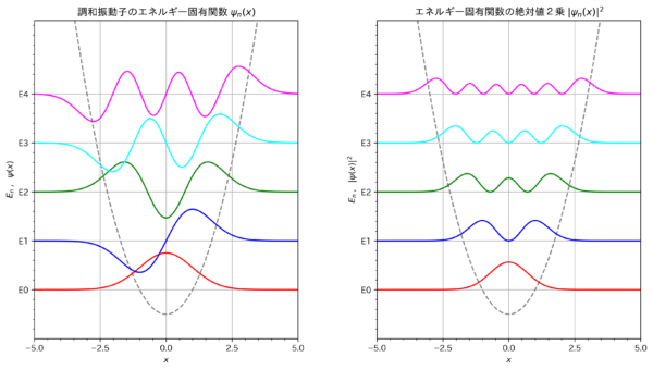
図 1. 調和振動子のエネルギー固有関数とその絶対値の2乗.
このグラフ化の Python ソースコードを以下に示しておく [2]ただし, Google Colaboratory で実行する場合, このままではフォントエラーが発生し日本語がきちんと表示されない.その場合は, … Continue reading .
import numpy as np
import math
import matplotlib.pyplot as plt
# Google Colaboratory で実行する場合は, 下行先頭の#を外すこと.
#import japanize_matplotlib

%matplotlib inline

amp = math.pow(math.pi, -1/4)

x = np.arange(-5, 5, 0.01)
y = amp*np.exp(-0.5*x*x)
y1 = y
y2 = math.sqrt(2)*x*y
y3 = (2*x*x-1)/math.sqrt(2)*y
y4 = (2*x**3-3*x)/math.sqrt(3)*y
y5 = (4*x**5-20*x**3+15*x)/math.sqrt(60)*y
y6 = (1024*x**10-23040*x**8+161280*x**6-403200*x**4+302400*x**2-30240)/math.sqrt(math.pow(2,10)*math.factorial(10))*y
vx = 1/2*x*x

fig,axes = plt.subplots(1, 2, figsize=(13, 7))

axes[0].plot(x, vx, linewidth=1.5, color="grey", linestyle="dashed")
axes[0].plot(x, y1+1/2, linewidth=1.5, color="red", label="n = 0")
axes[0].plot(x, y2+3/2, linewidth=1.5, color="blue", label="n = 1")
axes[0].plot(x, y3+5/2, linewidth=1.5, color="green", label="n = 2")
axes[0].plot(x, y4+7/2, linewidth=1.5, color="cyan", label="n = 3")
axes[0].plot(x, y5+9/2, linewidth=1.5, color="magenta", label="n = 4")

axes[1].plot(x, vx, linewidth=1.5, color="grey", linestyle="dashed")
axes[1].plot(x, y1*y1+1/2, linewidth=1.5, color="red", label="n = 0")
axes[1].plot(x, y2*y2+3/2, linewidth=1.5, color="blue", label="n = 1")
axes[1].plot(x, y3*y3+5/2, linewidth=1.5, color="green", label="n = 2")
axes[1].plot(x, y4*y4+7/2, linewidth=1.5, color="cyan", label="n = 3")
axes[1].plot(x, y5*y5+9/2, linewidth=1.5, color="magenta", label="n = 4")

# グラフのタイトル
axes[0].set_title(r"調和振動子のエネルギー固有関数 $\psi_n(x)$")
axes[1].set_title(r"エネルギー固有関数の絶対値2乗 $|\psi_n(x)|^{2}$")

# X軸の範囲の設定
axes[0].set_xlim(-5, 5)
axes[1].set_xlim(-5, 5)

# X軸のラベル
axes[0].set_xlabel("x")
axes[0].set_ylabel("$E_n$ , $\psi(x)$")
axes[0].set_ylim(-0.5, 6.0)
axes[1].set_xlabel("x")
axes[1].set_ylabel("$E_n$ , $|\psi(x)|^{2}$")
axes[1].set_ylim(-0.5, 6.0)
# 補助目盛りの描画
axes[0].minorticks_on()
axes[1].minorticks_on()
# 主目盛の設定
axes[0].set_xticks(np.linspace(-5, 5, 5))
axes[0].set_yticks(np.linspace(0.5, 4.5, 5))
axes[0].set_yticklabels(["E0", "E1","E2", "E3", "E4"])
axes[1].set_xticks(np.linspace(-5, 5, 5))
axes[1].set_yticks(np.linspace(0.5, 4.5, 5))
axes[1].set_yticklabels(["E0", "E1","E2", "E3", "E4"])

# 目盛り線の描画
axes[0].grid()
axes[1].grid()

# 凡例表示するには
#axes[0].legend(loc="upper right", bbox_to_anchor=(1,1))
#axes[1].legend(loc="upper right", bbox_to_anchor=(1,1))

# サブプロット間スペースの調整
fig.subplots_adjust(wspace=0.3)
plt.show()
また, 式 (7.49) の調和振動子固有状態, 及び式 (7.51) の任意関数として
\[ \psi(x)=\frac{1}{\sqrt{3}}\big\{ \phi_0(x)+\phi_1(x)+\phi_2(x)\big\} \]
の時間発展の様子をシミュレーションする Python アニメーションは例えば次のようである:
このアニメーションを見ると次のことが分かると思う:
「調和振動子のエネルギー固有関数は, 定常状態に相当するので, その時間変化は定常波となる.しかし, 幾つかのエネルギー固有関数を重ね合わせたものは, もはや定常状態の波動関数ではなく, その時間変化は進行波となる」.
このアニメーション化の Python ソースコードを以下に示しておく.
import numpy as np
import math
import matplotlib.pyplot as plt
# Google Colaboratory で実行する場合は, 次の行の先頭の # を外すこと.
#import japanize_matplotlib
from matplotlib import animation, rc
from IPython.display import HTML

fig, axes = plt.subplots(1, 2, figsize=(10, 5), constrained_layout=True)

# 各軸のラベル
# --> rを入れないとLaTeX出力されないので注意する.
axes[0].set_title(r"調和振動子のエネルギー固有関数 $\psi_n(x)$ の時間変化")
axes[1].set_title(r"$\psi(x)=(\psi_0(x)+\psi_1(x)+\psi_2(x))/\sqrt{3}$と$|\psi(x)|^{2}$の時間変化")
axes[0].set_xlabel(r"$x$", fontsize=15)
axes[0].set_ylabel(r"$\psi_0(x),\quad\psi_1(x),\quad\psi_2(x),\quad E_n$", fontsize=15)
axes[1].set_xlabel(r"$x$", fontsize=15)
axes[1].set_ylabel(r"$\psi(x),\quad |\psi(x)|^{2}$", fontsize=15)

# グラフの範囲を設定
axes[0].set_xlim([-4, 4])
axes[0].set_ylim([-0.5, 3.5])
axes[1].set_xlim([-4, 4])
axes[1].set_ylim([1, 5])
axes[0].set_xticks(np.linspace(-4, 4, 9))
axes[1].set_xticks(np.linspace(-4, 4, 9))
axes[0].set_yticks(np.linspace(0.5, 2.5, 3))
axes[0].set_yticklabels([r"$\hbar\omega/2$", r"$3\hbar\omega/2$", r"$5\hbar\omega/2$"])
axes[1].set_yticks(np.linspace(2.5, 4.5, 3))
axes[1].set_yticklabels([r"$5\hbar\omega/2$", r"$7\hbar\omega/2$", r"$9\hbar\omega/2$"])
axes[0].grid()
axes[1].grid()
#axes[1].legend()

# x点の計算範囲とその点数
x = np.linspace(-5, 5, 80)

amp = math.pow(math.pi, -1/4)
T=2*math.pi
dt=1/T
vx = 1/2*x*x
axes[0].plot(x, vx, color='gray', linestyle="dashed")
axes[1].plot(x, vx, color='gray', linestyle="dashed")

ims=[]
for a in range(200):
    y1 = amp*np.exp(-0.5*x*x)*np.cos(1/2*dt*a)
    y2 = amp*np.exp(-0.5*x*x)*math.sqrt(2)*x*np.cos(3/2*dt*a)
    y3 = amp*np.exp(-0.5*x*x)*(2*x*x-1)/math.sqrt(2)*np.cos(5/2*dt*a)
    ytotal = (1/math.sqrt(3))*amp*np.exp(-0.5*x*x)*(np.cos(1/2*dt*a)\
             +math.sqrt(2)*x*np.cos(3/2*dt*a)+(2*x*x-1)/math.sqrt(2)*np.cos(5/2*dt*a))
    im1 = axes[0].plot(x, y1+0.5, color='red')
    im2 = axes[0].plot(x, y2+1.5, color='green')
    im3 = axes[0].plot(x, y3+2.5, color='blue')
    im4 = axes[1].plot(x, ytotal+3.5, alpha=1.0, color='brown', label=r"\psi(x)=\psi_0(x)+\psi_1(x)+\psi_2(x)")
    im5 = axes[1].plot(x, ytotal*ytotal+3.5, linewidth=8, alpha=0.5, color='magenta', label=r"|\psi(x)|^{2}")
    ims.append(im1+im2+im3+im4+im5)

# ArtistAnimationにfigオブジェクトとimsを代入してアニメーションを作成
anim = animation.ArtistAnimation(fig, ims, interval=70) # interval値でグラフの描画速度が決まる.
#anim.save('anim1.mp4')

# Jupyter notebookの場合は
#plt.show()

# Google Colaboratoryの場合必要
rc('animation', html='jshtml')
plt.close()
anim
References
| ↑1 | 「スケーリング」(scaling):(1) 系の振る舞いが物理量の絶対値だけでなく,相対的な大きさのみで決まること.特に2変数関数 \(f(x,y)\) が1変数 \(x/y\) だけの関数として表されること.(2) 物理量を適当なベキで組み合わせて無次元化した変数を用いて運動方程式を表すこと. |
|---|---|
| ↑2 | ただし, Google Colaboratory で実行する場合, このままではフォントエラーが発生し日本語がきちんと表示されない.その場合は, プログラム実行前にまず, 次を実行する:
!pip install japanize-matplotlib その後, プログラム中の5行目の先頭の#を消してその行を付加すること. アニメーションプログラムの方も同じ作業が必要である. |