\(\)
前述のブログに示した自由波束の時間発展の様子をシミュレーションして見た.Bernd Thaller : 「Visual Quantum Mechanics」と「Advanced Visual Quantum Mechanics」を参照して, その python プログラムを書く手順とその結果の動画を示しておく.
まずはシミュレーションプログラムを書くための予備知識を確認しておく.
Schrödinger 理論による時間発展
自由粒子のシュレディンガー方程式は,
\(
\def\ppdiff#1#2{\frac{\partial #1}{\partial #2}}
\def\pdiff#1{\frac{\partial}{\partial #1}}
\def\Bppdiff#1#2{\frac{\partial^{2} #1}{\partial #2^{2}}}
\def\Bpdiff#1{\frac{\partial^{2}}{\partial #1^{2}}}
\def\mb#1{\mathbf{#1}}
\def\mr#1{\mathrm{#1}}
\def\reverse#1{\frac{1}{#1}}
\def\ds#1{\mbox{${\displaystyle\strut #1}$}}
\def\half{\frac{1}{2}}
\def\slashed#1{#1\llap{/}\,}
\def\slashW{W\!\!\llap{/}\,}
\def\BraKet#1#2#3{\left\langle #1 | #2 | #3 \right\rangle}
\def\BK#1#2{\left\langle #1 | #2 \right\rangle}
\)
i\hbar \pdiff{t}\psi(\mb{x},t)=-\frac{\hbar^{2}}{2m}\nabla^{2}\psi(\mb{x},t) = E\psi(\mb{x},t)
\tag{1}
\end{equation}
この平面波解は,
\psi(\mb{x},t)&=\exp\bigl\{i(\mb{k}\cdot\mb{x}-\omega t)\bigr\}
=\exp\left(\frac{i}{\hbar}\mb{p}\cdot\mb{x}-\frac{i}{\hbar}\frac{\mb{p}^{2}}{2m}t\right)\notag\\
&=\exp\left(-\frac{iEt}{\hbar}\right)\exp\left(i\frac{\sqrt{2mE}}{\hbar}\mb{x}\right)
\tag{2}
\end{align}
ただし,
\mb{p}=\hbar\mb{k},\quad |\mb{k}|=\frac{\sqrt{2mE}}{\hbar},\quad E=\hbar\omega=\frac{\mb{p}^{2}}{2m}=\frac{\hbar^{2}\mb{k}^{2}}{2m}
\tag{3}
\end{equation}
\(m=1\), \(\hbar=1\), \(c=1\) の単位系を用いたときの平面波解を \(u_{\mb{k}}(\mb{x},t)\) とすると,
u_{\mb{k}}(\mb{x},t) = \exp\left(i\mb{k}\cdot\mb{x}-i\frac{k^{2}}{2}t\right)
\tag{4}
\end{equation}
ただし \(E\) と \(\mb{k}\) の関係は次である:
E=E(\mb{k})=\frac{1}{2}\mb{k}^{2}
\tag{5}
\end{equation}
一般解 \(\psi\) は, 平面波解 \(u\) の重ね合わせによって表せるから,
\psi(\mb{x},t)= \frac{1}{(2\pi)^{n/2}}\int_{\mathbb{R}^{n}} \hat{\psi}_{0}(\mb{k})\,
e^{i\mb{k}\cdot\mb{x}-i\frac{k^{2}}{2}t}\,d^{n}k
=\frac{1}{(2\pi)^{n/2}}\int_{\mathbb{R}^{n}} e^{i\mb{k}\cdot\mb{x}}e^{-i\frac{k^{2}}{2}t}\hat{\psi}_{0}(\mb{k})
\,d^{n}k
\tag{6}
\end{equation}
従って \(\psi(\mb{x},t)\) は「 \(e^{i\frac{k^{2}}{2}t}\hat{\psi}_{0}(\mb{k})\) のフーリエ変換として得られる」と言える.
- 自由粒子の一般解を求める手順は次となる:
- 初期関数 \(\psi_{0}\) のフーリエ変換 \(\hat{\psi}\) を求める.
- \(\exp(-ik^{2}t/2)\hat{\psi}_0(\mb{k})\) の逆フーリエ変換を求める.
具体例として初期関数として, 任意定数 \(\alpha>0\), そして \(\mb{p}\in\mathbb{R}\) に対する次のガウス型関数の時間発展を求めてみよう.
\psi_{0}(x)=e^{ipx}e^{-\alpha x^{2}},\quad x \in \mathbb{R}
\tag{7}
\end{equation}
(第1ステップ) : この関数のフーリエ変換は次で与えられる:
\hat{\psi}_0(k)=\frac{1}{\sqrt{\alpha}}\exp\left\{-\frac{(k-p)^{2}}{2\alpha}\right\}
\tag{8}
\end{equation}
このとき, 関数 \(\psi_0\) の運動量 \(k\) は平均運動量 \(p\) の周りに分布している.
(第2ステップ) : 初期値問題の時間 \(t\) に於ける解は次で与えられる:
\psi(x,t)&= \frac{1}{\sqrt{2\pi}}\int e^{ikx}\frac{1}{\sqrt{\alpha}}e^{-ik^{2}t/2}
e^{-(k-p)^{2}/2\alpha}\,dk\\
&=\frac{1}{\sqrt{2\pi\alpha}}\exp\left(-\frac{p^{2}}{2\alpha}\right)
\int \exp\left\{-\frac{(it+1/\alpha)}{2}k^{2}+\left(ix+p/\alpha\right)k\right\}\,dk
\tag{9}
\end{align}
最後の積分中の指数関数は 次に書くことが出来る:
-\frac{it+1/\alpha}{2}q(k)^{2} + \frac{(ix+p/\alpha)^{2}}{2(it + 1/\alpha)},\quad
\mathrm{with}\quad q(k)=k-\frac{ix+p/\alpha}{it+1/\alpha}
\tag{10}
\end{equation}
従って \(\psi(x,t)\) は,
\psi(x,t)= \reverse{\sqrt{2\pi\alpha}}\exp\left\{-\frac{p^{2}}{2\alpha}
+ \frac{(ix+p/\alpha)^{2}}{2(it + 1/\alpha)}\right\}
\int \exp\left\{-(it+1/\alpha)\frac{q(k)^{2}}{2}\right\}\,dk
\tag{11}
\end{equation}
このとき,
\int \exp\left\{-(it+1/\alpha)\frac{q(k)^{2}}{2}\right\}\,dk
&=\int \exp\left\{-\frac{(it+1/\alpha)}{2}k^{2}\right\}\,dk
=\frac{\sqrt{2\pi}}{\sqrt{it + 1/\alpha}}\notag\\
&=\frac{\sqrt{2\pi\alpha}}{\sqrt{1+it\alpha}}
\tag{12}
\end{align}
よって \(\psi(x,t)\) は次のように書ける:
\psi(x,t)=\reverse{\sqrt{1+i\alpha t}}
\exp\left\{-\frac{\alpha x^{2} -2ixp + ip^{2}t}{2(1+i\alpha t)}\right\}
\tag{13}
\end{equation}
このとき, この指数関数の実部は 次のように書くことが出来る:
-\frac{\alpha}{2(1+\alpha^{2}t^{2})}(x-pt)^{2}
\tag{14}
\end{equation}
従って, 時間 \(t\) に於けるガウス波束の絶対値は やはりガウス関数である:
|\psi(x,t)| = (1+\alpha^{2}t^{2})^{-1/4}\exp\left\{-\frac{\alpha(t)}{2} (x-pt)^{2}\right\},\quad
\mathrm{where}\quad \alpha(t)=\frac{\alpha}{1+\alpha^{2}t^{2}}
\tag{15}
\end{equation}
ガウス関数 \(|\psi(x,t)|\) 及び確率密度 \(\rho=|\psi(x,t)|^{2}\) は, 位置 \(x(t)=pt\) を中心として拡がっている.それは質量 \(m=1\) で運動量 \(p\) を持った粒子が初期条件 \(x(0)=0\) で運動するときの, ちょうど時刻 \(t\) に於ける位置である.時刻 \(t\) に於けるガウス関数の拡がりは \(1/\sqrt{\alpha(t)}\) で与えられ, おおよそ \(t\) のように増大する.これは「波束の拡がり」と呼ばれる.またそれと同時に, 波束の最大値は \(1/\sqrt{t}\) のように減少する.
Dirac 理論による自由粒子波束の時間発展
時間依存する自由粒子の Dirac 方程式は, 前述の Schrödinger 理論と全く同じ仕方で解くことが出来る.まず, 二乗可積の初期スピノルとして 例えば,
\psi(x,t=0)=\phi(x)=\begin{pmatrix} \phi_1(x) \\ \phi_2(x) \end{pmatrix}
=\left(\frac{1}{32\pi}\right)^{1/4}\exp\left(-\frac{x^{2}}{16}\right)
\begin{pmatrix} 1 \\ 1 \end{pmatrix}
\tag{16}
\end{equation}
のフーリエ変換 \(\mathcal{F}\) を行う.その結果, 運動量空間に於ける二乗可積スピノル \(\hat{\phi}(k)\) が得られる:
\hat{\phi}(k)= \frac{1}{\sqrt{2\pi}}\int_{\mathbb{R}} e^{-ikx}\phi(x)\,dx
\tag{17}
\end{equation}
次に, この列ベクトルを基礎スピノル \(u_{\mr{pos}}(k)\) と \(u_{\mr{neg}}(k)\) の線形結合として書く:
\hat{\phi}(k)= \hat{\phi}^{+}(k)\,u_{\mr{pos}}(k) + \hat{\phi}^{-}(k)\,u_{\mr{neg}}(k)
\tag{18}
\end{equation}
ここで展開係数 \(\hat{\phi}^{\pm}(k)\) は \(\mathbb{C}^{2}\) スカラー積によって与えられる (下の式 (24) を参照):
\hat{\phi}^{+}(k)= \langle u_{\mr{pos}}(k),\hat{\phi}(k)\rangle_{2}
&=\overline{u_{\mr{pos}}(k)}_{1}\,\hat{\phi}_{1}(k) + \overline{(u_{\mr{pos}})}_{2}\,\hat{\phi}_{2}(k)
=\overline{d_{+}(k)}\,\hat{\phi}_{1}(k) + \overline{d_{-}(k)}_{2}\,\hat{\phi}_{2}(k),\\
\hat{\phi}^{-}(k)= \langle u_{\mr{neg}}(k),\hat{\phi}(k)\rangle_{2}
&=\overline{(u_{\mr{neg}})}_{1}\,\hat{\phi}_{1}(k) + \overline{(u_{\mr{neg}})}_{2}\,\hat{\phi}_{2}(k)
=-\overline{d_{-}(k)}\,\hat{\phi}_{1}(k) + \overline{d_{+}(k)}_{2}\,\hat{\phi}_{2}(k)
\tag{19}
\end{align}
運動量空間に於ける自由粒子の Dirac 演算子 \(H_{0}\) の作用 \(\mb{h}_{0}(k)\) は,
\mb{h}_{0}(k)=c\alpha k + \beta mc^{2} =\begin{pmatrix} mc^{2} & ck \\ ck & -mc^{2} \end{pmatrix}
\tag{20}
\end{equation}
で与えられ, その固有値は次である:
\lambda(k)=\sqrt{c^{2}k^{2}+m^{2}c^{4}}
\tag{21}
\end{equation}
\(d_{+}(k)\) と \(d_{-}(k)\) を, この \(\mb{h}_{0}(k)\) を対角化するユニタリー行列 \(\mb{u}(k)\) の係数とする:
\mb{u}(k)= d_{+}(k)\mb{1}_{2}\ +\ d_{-}(k)\,\beta\alpha
\tag{22}
\end{equation}
すると \(\mb{u}^{\dagger}(k)\) を構成する列ベクトルが, 行列 \(\mb{h}_{0}(k)\) の固有ベクトルとなる:
\mb{u}^{\dagger}(k)= d_{+}(k)\mb{1}_{2}\ -\ i d_{-}(k)\,\sigma_{2}
\tag{23}
\end{equation}
従って, 正の固有値 \(+\lambda(k)\) に属する固有ベクトル \(u_{\mr{pos}}(k)\) と, 負の固有値 \(-\lambda(k)\) に属する固有ベクトル \(u_{\mr{neg}}(k)\) は次となる:
u_{\mr{pos}}(k)=\mb{u}^{\dagger}(k)\begin{pmatrix} 1 \\ 0 \end{pmatrix}
=\begin{pmatrix} d_{+}(k) \\ d_{-}(k) \end{pmatrix},\quad
u_{\mr{neg}}(k)=\mb{u}^{\dagger}(k)\begin{pmatrix} 0 \\ 1 \end{pmatrix}
=\begin{pmatrix} -d_{-}(k) \\ d_{+}(k) \end{pmatrix}
\tag{24}
\end{equation}
次のステップは, 式 (18) の \(\hat{\phi}(k)\) 部分に 時間因子 \(\exp(\mp i\lambda(k)t)\) を掛け合わせることである:
\hat{\psi}(k,t)= \hat{\phi}^{+}(k)\,u_{\mr{pos}}(k)\,e^{-i\lambda(k)t}
+ \hat{\phi}^{-}(k)\,u_{\mr{neg}}(k)\,e^{i\lambda(k)t}
\tag{25}
\end{equation}
最後に, この \(\hat{\psi}(k,t)\) を「逆フーリエ変換」する:
\psi(x,t)&=\frac{1}{\sqrt{2\pi}}\int_{\mathbb{R}} e^{ikx}\hat{\psi}(k,t)\,dk\notag\\
&=\int_{\mathbb{R}} \left\{\hat{\phi}^{+}(k)\,\frac{1}{\sqrt{2\pi}}u_{\mr{pos}}(k)\,e^{ikx -i\lambda(k)t}
+ \hat{\phi}^{-}(k)\,\frac{1}{\sqrt{2\pi}}u_{\mr{neg}}(k)\,e^{ikx + i\lambda(k)t}
\right\}\,dk\notag\\
&= \int_{\mathbb{R}} \left\{\hat{\phi}^{+}(k)\,u_{\mr{pos}}(k;x,t)+
\hat{\phi}^{-}(k)\,u_{\mr{neg}}(k;x,t)\right\}\,dk
\tag{26}
\end{align}
ただし, 最後の段階の \(u_{\mr{pos}}(k;x,t)\) と \(u_{\mr{neg}}(k;x,t)\) は, 自由粒子に対する Dirac 方程式の平面波解である:
u_{\mr{pos}}(k;x,t)=\frac{1}{\sqrt{2\pi}}u_{\mr{pos}}(k)\,e^{ikx -i\lambda(k)t},\quad
u_{\mr{neg}}(k;x,t)=\frac{1}{\sqrt{2\pi}}u_{\mr{neg}}(k)\,e^{ikx + i\lambda(k)t}
\tag{27}
\end{equation}
この式 (27) によって, 初期状態がガウス波束 \(\phi\) の場合に於ける「時間依存する自由 Dirac 方程式 解」が得られたことになる.
複素数値関数の可視化
ここでは複素数を可視化するのに「位相」をカラーコードで表す方法を用いる.それは, 位置 \(x\) に於ける(複素数値を持つ)「波動関数の絶対値」はプロットで示し,「位相」を示すにはそのグラフと \(x\) 軸間の領域を「波動関数の位相に対応したカラーマップの色」で塗り潰すやり方である.カラーマップは HSV を用いる.詳しくは B.Thaller :「Visual Quantum Mechanics」の第 1 章を参照すべし.
シミュレーションプログラムとその結果
最初に Schrödinger 理論による時間発展のシミュレーションプログラムとその結果を示す.以下の python プログラムは全て, 今流行の生成 AI に書いてもらった.
import numpy as np
import matplotlib.pyplot as plt
import matplotlib.animation as animation
from matplotlib import cm

# Define the function Psi
def Psi(x, t, a, p):
return (1 / np.sqrt(1 + 1j * a * t)) * np.exp(-(a * x**2 - 2 * 1j * x * p + 1j * p**2 * t) / (2 * (1 + 1j * a * t)))

# Define the ColorFunction
def color_function(x, t, a, p):
return cm.hsv(np.mod(np.angle(Psi(x, t, a, p)), 2 * np.pi) / (2 * np.pi))

# Set up the figure and axis
fig, ax = plt.subplots(figsize=(8, 6))
x = np.linspace(-10, 30, 400)
a = 1/16
p = 3/4
t_values = np.linspace(0, 50, 300) # Time values for animation

# Initialize plot elements
line, = ax.plot(x, np.abs(Psi(x, 0, a, p)), lw=2) # Initialize with t=0 data
ax.set_xlim([-10, 30])
ax.set_ylim([0, 1.05])
ax.set_xlabel(r'$x$')
ax.set_ylabel(r'$|\psi(x)|$')
plt.title("Time Evolution of " r'$|\psi(x, t)|$')

# Initial fill with colors
fill_collections = []
for i in range(len(x) - 1):
x_fill = [x[i], x[i+1]]
y_fill = [np.abs(Psi(x[i], 0, a, p)), np.abs(Psi(x[i+1], 0, a, p))]
fill = ax.fill_between(x_fill, y_fill, 0, color=color_function(x[i], 0, a, p), alpha=0.7)
fill_collections.append(fill)

def update(frame):
t = t_values[frame]
y = np.abs(Psi(x, t, a, p))
line.set_data(x, y)

# Remove previous fills
for fill in fill_collections:
fill.remove()
fill_collections.clear()

# Update fill colors
for i in range(len(x) - 1):
x_fill = [x[i], x[i+1]]
y_fill = [y[i], y[i+1]]
fill = ax.fill_between(x_fill, y_fill, 0, color=color_function(x[i], t, a, p), alpha=0.7)
fill_collections.append(fill)

return line,

# Create animation
ani = animation.FuncAnimation(fig, update, frames=len(t_values), blit=False, interval=50)

# Save animation as GIF
ani.save("Psi_wave3.gif", writer="pillow", fps=20)

plt.show()
出力されたシミュレーション動画は次である:
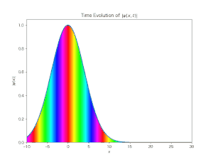
図 1. ガウス波束の時間発展を Schrödinger 理論によってシミュレーションしたグラフ
このグラフの色と偏角との関係は, 次のカラーマップによって配色されている:
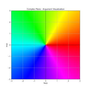
図 2. 複素平面のカラーマップ
この図もやはり生成AIの助けを借りて書いたものである.上記本のカラーページに載っていた図を生成AIに与え,「これと同じグラフを書いて」とお願いするだけであった.
次は同様なガウス波束を, 今度は Dirac 理論によってシミュレーションしたプログラムを示す:
import matplotlib
matplotlib.use('TkAgg')
import numpy as np
import scipy.integrate as integrate
import matplotlib.pyplot as plt
import matplotlib.animation as animation
def La(k):
return np.sqrt(k**2 + 1)
def dp(k):
return np.sqrt(1 + 1/La(k)) / np.sqrt(2)
def dm(k):
return np.sign(k) * np.sqrt(1 - 1/La(k)) / np.sqrt(2)
def b(k):
return (2/np.pi)**(1/4) * np.exp(-4 * (k-3/4)**2) * (dp(k) + dm(k))
def d(k):
return (2/np.pi)**(1/4) * np.exp(-4 * (k-3/4)**2) * (dp(k) - dm(k))
def up1(k, x, t):
return dp(k) / np.sqrt(2) * np.exp(1j * k * x - 1j * La(k) * t)
def up2(k, x, t):
return dm(k) / np.sqrt(2) * np.exp(1j * k * x - 1j * La(k) * t)
def um1(k, x, t):
return -dm(k) / np.sqrt(2) * np.exp(1j * k * x + 1j * La(k) * t)
def um2(k, x, t):
return dp(k) / np.sqrt(2) * np.exp(1j * k * x + 1j * La(k) * t)
def psi1(x, t):
def integrand_real(k):
return np.real(b(k) * up1(k, x, t) + d(k) * um1(k, x, t))
def integrand_imag(k):
return np.imag(b(k) * up1(k, x, t) + d(k) * um1(k, x, t))
result_real, _ = integrate.quad(integrand_real, -np.inf, np.inf, epsabs=1e-3, epsrel=1e-3)
result_imag, _ = integrate.quad(integrand_imag, -np.inf, np.inf, epsabs=1e-3, epsrel=1e-3)
return result_real + 1j * result_imag
def psi2(x, t):
def integrand_real(k):
return np.real(b(k) * up2(k, x, t) + d(k) * um2(k, x, t))
def integrand_imag(k):
return np.imag(b(k) * up2(k, x, t) + d(k) * um2(k, x, t))
result_real, _ = integrate.quad(integrand_real, -np.inf, np.inf, epsabs=1e-3, epsrel=1e-3)
result_imag, _ = integrate.quad(integrand_imag, -np.inf, np.inf, epsabs=1e-3, epsrel=1e-3)
return result_real + 1j * result_imag
def rho(x, t):
return np.abs(psi1(x, t))**2 + np.abs(psi2(x, t))**2
x_values = np.linspace(-20, 20, 100)
times = np.linspace(0, 30, 300)
fig, ax = plt.subplots()
ax.set_xlim(-20, 20)
ax.set_ylim(-0.5, 1)
ax.grid()
ax.set_xlabel(r'$x$')
ax.set_ylabel(r'$\rho(x)$')
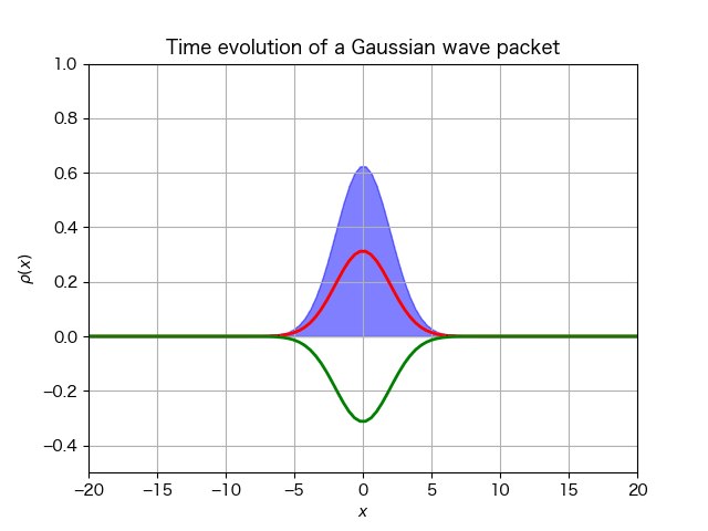
ax.set_title("Time evolution of a Gaussian wave packet with positive momentum")
fill = ax.fill_between(x_values, np.zeros_like(x_values), np.zeros_like(x_values), color='blue', alpha=0.5)
line1, = ax.plot([], [], color='red', lw=2) # Line for y_psi1
line2, = ax.plot([], [], color='green', lw=2) # Line for y_psi2
def animate(t):
y_rho = [rho(x, t) for x in x_values]
y_psi1 = [np.abs(psi1(x, t))**2 for x in x_values]
y_psi2 = [-1*np.abs(psi2(x, t))**2 for x in x_values]
global fill
fill.remove()
fill = ax.fill_between(x_values, 0, y_rho, color='blue', alpha=0.5)
line1.set_data(x_values, y_psi1)
line2.set_data(x_values, y_psi2)
return fill, line1, line2
ani = animation.FuncAnimation(fig, animate, frames=times, interval=20, blit=False, repeat=False)
ani.save("wave_packet_momentum.gif", writer="pillow") # gif動画として保存する.
#plt.show() # 表示もさせたいならコメントアウトのマークを外す.
print("Program is finished!")
この場合, 数値積分の計算などを何回も行うので動画作成に時間がだいぶ掛かってしまう(非力のMac miniでは30分前後掛かった).
そのため cython を導入して高速化してみた.以下は生成AIの指示である:
【準備】
(1) まず Cython用の .pyx ファイル: wave_packet.pyx (Cythonコード)を作成します:
#
# wave_packet.pyx
#

# distutils: language = c
# cython: boundscheck=False, wraparound=False, nonecheck=False, cdivision=True

import numpy as np
cimport numpy as cnp
from scipy.integrate import quad
cimport cython
from libc.math cimport sqrt, exp, sin, cos

cdef double La(double k):
    return sqrt(k * k + 1)

cdef double dp(double k):
    return sqrt(1 + 1/La(k)) / sqrt(2)

cdef double dm(double k):
    return (1 if k >= 0 else -1) * sqrt(1 - 1/La(k)) / sqrt(2)

cdef double complex up1(double k, double x, double t):
    cdef double complex phase = cos(k*x - La(k)*t) + 1j*sin(k*x - La(k)*t)
    return dp(k) / sqrt(2) * phase

cdef double complex up2(double k, double x, double t):
    cdef double complex phase = cos(k*x - La(k)*t) + 1j*sin(k*x - La(k)*t)
    return dm(k) / sqrt(2) * phase

cdef double complex um1(double k, double x, double t):
    cdef double complex phase = cos(k*x + La(k)*t) + 1j*sin(k*x + La(k)*t)
    return -dm(k) / sqrt(2) * phase

cdef double complex um2(double k, double x, double t):
    cdef double complex phase = cos(k*x + La(k)*t) + 1j*sin(k*x + La(k)*t)
    return dp(k) / sqrt(2) * phase

cdef double complex b(double k):
    """ Computes the function b(k) """
    cdef double norm = (2/3.141592653589793)**0.25
    return norm * exp(-4 * (k - 0.75)**2) * (dp(k) + dm(k))

cdef double complex d(double k):
    """ Computes the function d(k) """
    cdef double norm = (2/3.141592653589793)**0.25
    return norm * exp(-4 * (k - 0.75)**2) * (dp(k) - dm(k))

@cython.boundscheck(False)
@cython.wraparound(False)
def psi1(double x, double t):
    """ Compute psi1 using numerical integration """
    cdef double result_real, result_imag
    result_real, _ = quad(lambda k: (b(k) * up1(k, x, t) + d(k) * um1(k, x, t)).real, -10, 10, epsabs=1e-3, epsrel=1e-3)
    result_imag, _ = quad(lambda k: (b(k) * up1(k, x, t) + d(k) * um1(k, x, t)).imag, -10, 10, epsabs=1e-3, epsrel=1e-3)
    return result_real + 1j * result_imag

@cython.boundscheck(False)
@cython.wraparound(False)
def psi2(double x, double t):
    """ Compute psi2 using numerical integration """
    cdef double result_real, result_imag
    result_real, _ = quad(lambda k: (b(k) * up2(k, x, t) + d(k) * um2(k, x, t)).real, -10, 10, epsabs=1e-3, epsrel=1e-3)
    result_imag, _ = quad(lambda k: (b(k) * up2(k, x, t) + d(k) * um2(k, x, t)).imag, -10, 10, epsabs=1e-3, epsrel=1e-3)
    return result_real + 1j * result_imag

@cython.boundscheck(False)
@cython.wraparound(False)
def rho(double x, double t):
    """ Compute probability density """
    return abs(psi1(x, t))**2 + abs(psi2(x, t))**2
(2) Cythonコンパイル用 setup.py を作成します:
#
# setup.py
#
from setuptools import setup, Extension
from Cython.Build import cythonize
import numpy

ext_modules = [
    Extension(
        "wave_packet",
        ["wave_packet.pyx"],
        include_dirs=[numpy.get_include()],
        define_macros=[("NPY_NO_DEPRECATED_API", "NPY_1_7_API_VERSION")],
    )
]

setup(
    ext_modules=cythonize(ext_modules, language_level=3, annotate=True),
)
(3) Pythonスクリプト main.py を作成します:
#
# main.py
#
import numpy as np
import matplotlib.pyplot as plt
import matplotlib.animation as animation
from wave_packet import psi1, psi2, rho

x_values = np.linspace(-20, 20, 100)
times = np.linspace(0, 30, 300)

fig, ax = plt.subplots()
ax.set_xlim(-20, 20)
ax.set_ylim(-0.5, 1)
ax.grid()
ax.set_xlabel(r'$x$')
ax.set_ylabel(r'$\rho(x)$')
ax.set_title("Time evolution of a Gaussian wave packet with positive momentum")

fill = ax.fill_between(x_values, np.zeros_like(x_values), np.zeros_like(x_values), color='blue', alpha=0.5)
line1, = ax.plot([], [], color='red', lw=2)
line2, = ax.plot([], [], color='green', lw=2)

def animate(t):
    y_rho = np.array([rho(x, t) for x in x_values])
    y_psi1 = np.array([abs(psi1(x, t))**2 for x in x_values])
    y_psi2 = -1 * np.array([abs(psi2(x, t))**2 for x in x_values])
    global fill
    fill.remove()
    fill = ax.fill_between(x_values, 0, y_rho, color='blue', alpha=0.5)
    line1.set_data(x_values, y_psi1)
    line2.set_data(x_values, y_psi2)
    return fill, line1, line2

ani = animation.FuncAnimation(fig, animate, frames=times, interval=20, blit=False, repeat=False)
ani.save("wave_packet_momentum.gif", writer="pillow")
print("Program is finished!")
【使い方】
1. Cythonコードをコンパイルします(ターミナルで):
python setup.py build_ext --inplace2. Pythonスクリプト (main.py) を実行します(ターミナルで):
python main.pyこの結果, 動画作成に掛かった時間は約30秒となった!.
シミュレーション結果は次である:
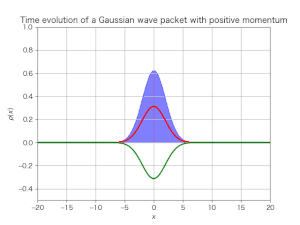
図 3. ディラック理論によるガウス波束の時間発展
今度はディラックスピノルの絶対値 \(|\psi(x,t)|\) だけでなく, スピノルの正エネルギー成分の絶対値 \(|\psi_{1}|\) と負エネルギー成分の絶対値 \(|\psi_{2}|\) も一緒に表示されている.色で塗られているのが \(|\psi(x,t)|\) である(今度は偏角のカラー表示はしていない).負エネルギー成分は \(x\) 軸の下に反転して描かれているので注意するべし.また, ときどき角のようなスパイクが見られるが, これはプログラムの計算誤差によるものである.プログラム中の数値などをキチンと調整すれば無くなると思う.左右の揺れである「Zitterbewegung」現象は初期の頃だけで見られる.
参考のために「初期状態で静止しているガウス波束の時間発展」の様子をシミュレーションした動画も示しておこう.左右に細かく揺れていて「Zitterbewegung」現象の存在がよく分かると思う:
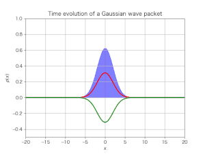
図 4. 静止したガウス波束の時間発展