コヒーレント状態の時間変化

前述した「コヒーレント状態」の波動関数は,「形が拡がらずに前後に運動する波束となる」ことが期待される．実際, コヒーレント状態の波動関数は, そのような時間変化をするであろうか？．詳しく調べて見よう．

前述のブログ記事から, $| α ⟩$ の時間発展は次であった：

\begin{aligned} (3.117) & e^{- i \hat{H} t / ℏ} | α ⟩ & = e^{- \frac{| α |^{2}}{2}} \sum_{n} \frac{α^{n}}{\sqrt{n!}} e^{- i (n + \frac{1}{2}) ω t} | n ⟩ = e^{i \frac{1}{2} ω t} e^{- \frac{| α |^{2}}{2}} \sum_{n} \frac{(α e^{- i ω t})^{n}}{\sqrt{n!}} | n ⟩ \end{aligned}

また, 個数状態の波動関数

ψ_{n} (q) = ⟨ q | n ⟩

の具体的な形は次であった：

\begin{matrix} (1) & ψ_{n} (q) = ⟨ q | n ⟩ = \frac{1}{π^{1 / 4} \sqrt{2^{n} n!}} \exp (- \frac{q^{2}}{2}) H_{n} (q) \end{matrix}

従って, 上式 (3.117) に左から

⟨ q |

を掛け合わせ, 式 (1) を代入することで, コヒーレント状態の波動関数

ψ_{α} (q, t)

は次のように求まる：

\begin{aligned} ψ_{α} (q, t) & = ⟨ q | e^{- i \hat{H} t / ℏ} | α ⟩ = e^{i \frac{1}{2} ω t} e^{- \frac{| α |^{2}}{2}} \sum_{n} \frac{(α e^{- i ω t})^{n}}{\sqrt{n!}} ⟨ q | n ⟩ \\ = e^{i \frac{1}{2} ω t} e^{- \frac{| α |^{2}}{2}} \sum_{n} \frac{α^{n} e^{- i n ω t}}{\sqrt{n!}} \cdot \frac{1}{π^{1 / 4} \sqrt{2^{n} n!}} e^{- \frac{q^{2}}{2}} H_{n} (q) \\ = e^{i \frac{1}{2} ω t} e^{- \frac{| α |^{2}}{2}} e^{- \frac{q^{2}}{2}} \frac{1}{π^{1 / 4}} \sum_{n} \frac{α^{n} e^{- i n ω t}}{\sqrt{2^{n}} n!} H_{n} (q) \end{aligned}

ここで, 一般に

α

は複素数であるから

α = | α | e^{i ϕ}

として次と置く：

\begin{matrix} (2) & z \equiv \frac{α e^{- i ω t}}{\sqrt{2}} = \frac{| α | e^{- i (ω t - ϕ)}}{\sqrt{2}}, \to z^{n} = \frac{α^{n} e^{- i n ω t}}{\sqrt{2^{n}}} \end{matrix}

すると上式は次に書ける：

\begin{matrix} (3) & ψ_{α} (q, t) = e^{i \frac{1}{2} ω t} e^{- \frac{| α |^{2}}{2}} e^{- \frac{q^{2}}{2}} \frac{1}{π^{1 / 4}} \sum_{n} \frac{z^{n}}{n!} H_{n} (q) \end{matrix}

ここで更に,「エルミート多項式の母関数( generating function )」

S (q, s)

を利用する：

\begin{matrix} (4) & S (q, s) \equiv e^{q^{2} - (s - q)^{2}} = \sum_{n = 0}^{\infty} \frac{H_{n} (q)}{n!} s^{n} \end{matrix}

このときの

s

は「補助変数」と呼ばれる．すると式 (3) の最後の部分は, ちょうど補助変数

s = z

の場合になっている!．よって, 式 (2) も用いることで式 (3) は次のように書ける：

\begin{aligned} ψ_{α} (q, t) = e^{i \frac{1}{2} ω t} e^{- \frac{| α |^{2}}{2}} e^{- \frac{q^{2}}{2}} \frac{1}{π^{1 / 4}} e^{q^{2} - (z - q)^{2}} \\ = \frac{1}{π^{1 / 4}} \exp (i \frac{1}{2} ω t) \exp [- \frac{1}{2} q^{2} + 2 z q - z^{2} - \frac{| α |^{2}}{2}] \\ = \frac{1}{π^{1 / 4}} \exp (i \frac{1}{2} ω t) \exp [- \frac{q^{2}}{2} + \sqrt{2} | α | q e^{- i (ω t - ϕ)} - \frac{| α |^{2}}{2} {1 + e^{- i 2 (ω t - ϕ)}}] \\ = \frac{1}{π^{1 / 4}} \exp (i \frac{1}{2} ω t) \exp [- \frac{q^{2}}{2} + \sqrt{2} | α | q \cos (ω t - ϕ) - \frac{| α |^{2}}{2} {1 + \cos 2 (ω t - ϕ)}] \\ \times \exp [- i \sqrt{2} | α | q \sin (ω t - ϕ) + i \frac{| α |^{2}}{2} \sin 2 (ω t - ϕ)] \\ = \frac{1}{π^{1 / 4}} \exp (i \frac{1}{2} ω t) \exp [- \frac{q^{2}}{2} + \sqrt{2} | α | q \cos (ω t - ϕ) - | α |^{2} \cos^{2} (ω t - ϕ)] \\ \times \exp [- i \sqrt{2} | α | q \sin (ω t - ϕ) + i | α |^{2} \sin (ω t - ϕ) \cos (ω t - ϕ)] \\ = \frac{1}{π^{1 / 4}} \exp (i \frac{1}{2} ω t) \exp [- \frac{1}{2} {q - \sqrt{2} | α | \cos (ω t - ϕ)}^{2}] \\ (5) & \times \exp [- i \sqrt{2} | α | q \sin (ω t - ϕ) + i | α |^{2} \sin (ω t - ϕ) \cos (ω t - ϕ)] \end{aligned}

従って, 確率密度

| ψ_{α} (q) |^{2}

は次のように書ける：

\begin{matrix} (6) & | ψ_{α} (q) |^{2} = \frac{1}{\sqrt{π}} \exp [- {x - λ \cos (ω t - ϕ)}^{2}], λ \equiv \sqrt{2} | α | \end{matrix}

これは,『確率密度関数はガウス波束であり, その中心が「振幅が

λ = \sqrt{2} α

である古典的な調和振動子の軌道

y = λ \cos (ω t - ϕ)

と同じ調和振動をする」ことを示している！』．そして普通ならば, 波束は時間と共に拡がることが予期されるのであるが, この特別な波束は「時間が経っても形を変えない！」ことも分かる．
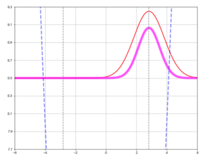
このことを示すために, 式 (5) の「コヒーレント状態の波動関数」

ψ_{α} (q)

の実数部分および式 (6) の「コヒーレント状態の確率密度」

| ψ_{α} (q) |^{2}

を, 固有値

α = 2

の場合でシミュレーレートするアニメーション, 及びその Python プログラムを以下に示しておく．アニメーション中, 赤線は波動関数の実数部分を表しており, 桃色の太線が確率密度関数である．

import numpy as np
import math
import matplotlib.pyplot as plt
from matplotlib import animation, rc
from IPython.display import HTML
 
# Figureのインスタンス生成
fig, axe = plt.subplots(1, 1, figsize=(10, 8))
 
amp = math.pow(math.pi, -1/4)
alpha =2
dt=1/25
T=2*math.pi/dt
time = math.ceil(2*T)
x0 = alpha*math.sqrt(2)
x = np.linspace(-6, 6, 400)
sift=x0*x0+0.5
 
ims = []
for t in range(time):
    pt= -x0*math.sin(t*dt)
    xt= x0*math.cos(t*dt)
    y = amp*np.exp(-1.j*pt*xt/2-1.j*t*dt/2)*np.exp(pt*x*1.j-(x-xt)**2/2)
    yy = np.conj(y)*y
    im1 = axe.plot(x, y.real+sift, linewidth=2, color='red')
    im2 = axe.plot(x, yy.real+sift, linewidth=7, alpha=0.7, color='magenta')
    ims.append(im1+im2)
 
anim = animation.ArtistAnimation(fig, ims, interval=80)
 
# 全エネルギー E=T+V+0.5=2V+0.5=2*V(a)+0.5=2*(sqrt(2)*alpha)^2+0.5=2*alpha^2+0.5,
hy = 1/2*x*x # harmonic potential V(x)=x^2/2,  
axe.plot(x,hy, color='blue', linewidth=3, alpha=0.5, linestyle="--")
rectangle = 10*np.heaviside(x+alpha*math.sqrt(2),4.5)-10*np.heaviside(x-alpha*math.sqrt(2),4.5)
axe.plot(x, rectangle, color='gray', linestyle="--") # ground state is sifted a=sqrt(2)*alpha
 
axe.set_xlim([-6, 6])
axe.set_ylim([sift-0.8, sift+0.8]) 
axe.set_yticks([7.7, 7.9, 8.1, 8.3, 8.5, 8.7, 8.9, 9.1, 9.3])
axe.grid()
#axe.legend()
# Jupyter notebookの場合は
#plt.show()
 
# Google Colaboratoryの場合必要
rc('animation', html='jshtml')
plt.close()
anim

【補足】波動関数の周期的な時間依存性

複素数であるコヒーレント状態の波動関数 $ψ_{α} (q, t)$ は, カラー表示を利用することで表すことが出来るようだ．
そこで Wolfram Cloud によって, 複素数である式 (5) のコヒーレント状態波動関数をカラー表示でグラフ化したものを示しておく：

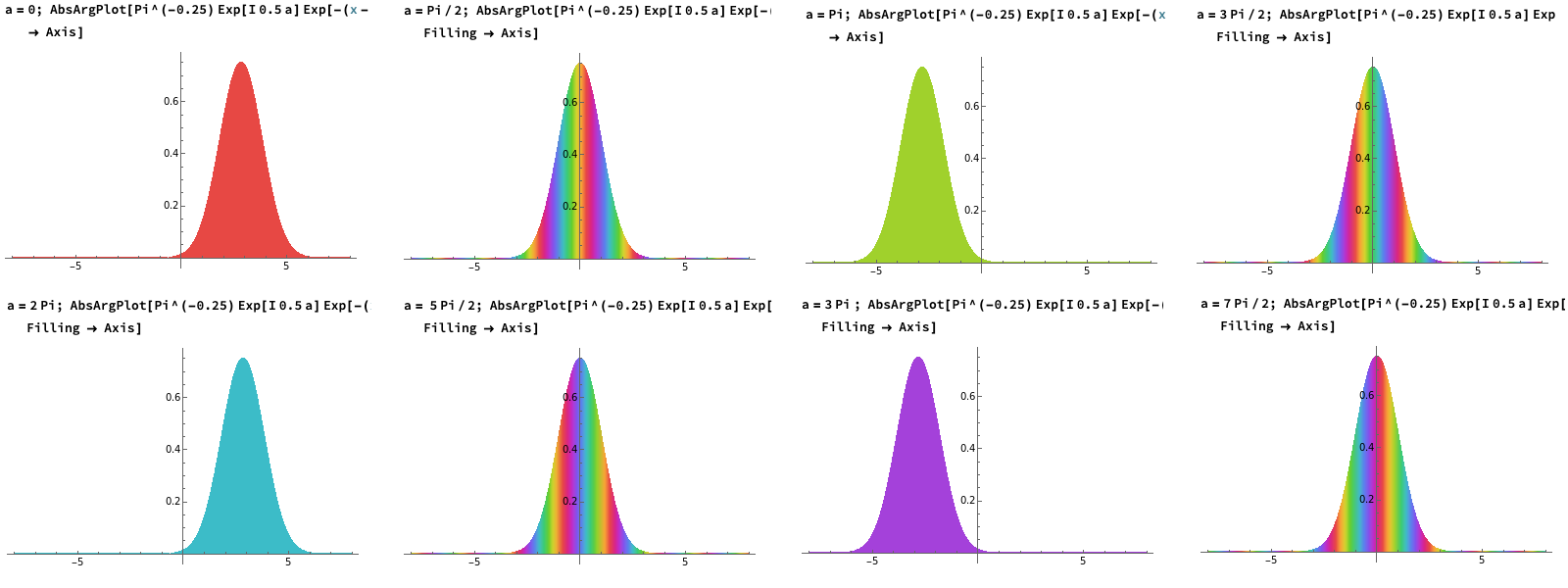
図 1. 複素数のカラー表示手法によって, コヒーレント状態の波動関数 $ψ_{α} (q, t)$ の時間変化を時間間隔 $Δ a = p i / 2$ ごとに描いたもの．波動関数の絶対値 $| ψ_{α} (q, t) |$ はその波形で表わされ, その位相部分(偏角)はカラー(色)によって表わされている．従って, 端点の波束中で偏角が変化していない場合には純色である．しかし, 偏角が変化し振動している場合には, 色が変化するので虹色模様になっているのが分かる．

図は時間間隔 $Δ a = π / 2$ ごとに描いたものである．これを見ると,「波動関数の絶対値 $| ψ_{α} (q, t) |$ の形は, 時間発展しても一定に保たれる」ことが確認される．しかし, 注意すべきは波動関数の位相を表現するその波形の色である．調和振動子の周期は $2 π$ であるが,「この量子力学的波動関数の周期は明らかにそうなっていない．実はその周期は $4 π$ となる」．そのことを「Visual Quantum Mechanics」の § 7.3.2 からの抜粋で記しておく．

7.3.2. 周期的な時間依存性

１次元調和振動子の量子力学的状態の時間発展は,「時間依存するシュレディンガー方程式」によって記述される：

\begin{matrix} (1) & i ℏ \frac{d}{d t} ψ (x, t) = H ψ (x, t), H = - \frac{ℏ}{2 m} \frac{d^{2}}{d x^{2}} + \frac{k}{2} x^{2} \end{matrix}

この方程式の一般解は, そのエネルギー固有関数

ϕ_{n} (x)

の重ね合わせとして表される：

\begin{matrix} (2) & ψ (x, t) = \sum_{n = 0}^{\infty} c_{n} e^{- i E_{n} t} ϕ_{n} (x) \end{matrix}

このとき, 式 (2) から次のことが言える：

【振動状態の時間対称性】
調和振動子ポテンシャルのシュレディンガー方程式の任意の解は次の特性を持つ：

$\begin{matrix} (7.53) & ψ (x, t + π) = e^{- i π / 2} ψ (- x, t) \end{matrix}$

従って,

$\begin{matrix} (7.54) & ψ (x, t + 2 π) = e^{- i π / 2} ψ (- x, t + π) = e^{- i π} ψ (x, t) = - ψ (x, t) \end{matrix}$

【振動状態の周期的な時間依存性】
全ての初期状態 $ϕ$ に対して, 式 (1) の解 $ψ (x, t)$ の周期は $T = 4 π$ である．しかし, 「波動関数」 $ψ$ の周期は $4 π$ であるけれども, 量子力学的「状態」(そして特に位置の確率密度 $| ψ (x, t) |^{2}$ ) の周期は $2 π$ となる．それは, 相当する古典力学系の周期に等しい．